Usage:

Pre-processing:

In order to use LONGO the data needs to be in a specific format. This format has the gene identifier in the first column and all of the other columns are expression values. The first row can be a header which will help in viewing the plots. An example data set can be downloaded here. This data is in the correct format.

LONGO():

The next step is to use the start the shiny interface of LONGO using: LONGO() This will start a new window showing the main menu as seen in figure 1.

figure 1

Once you have the session started you can upload your data file. For this example the dataset provided above is going to be used. The data file is for humans so the default species gene ensembl can be used. If your data is from a different species select it from the drop down. As you change the species the available options for the gene identifier will also change. This is because the biomart database has different identifiers for different species. The example data uses the affy_primeview as a gene identifier. The default option fo the separator is tab separated, which is what the example data file uses. Once all the correct options are selected the view should look like figure 2. As the options related to the data file are changed the updated view of the data is shown in the main window.

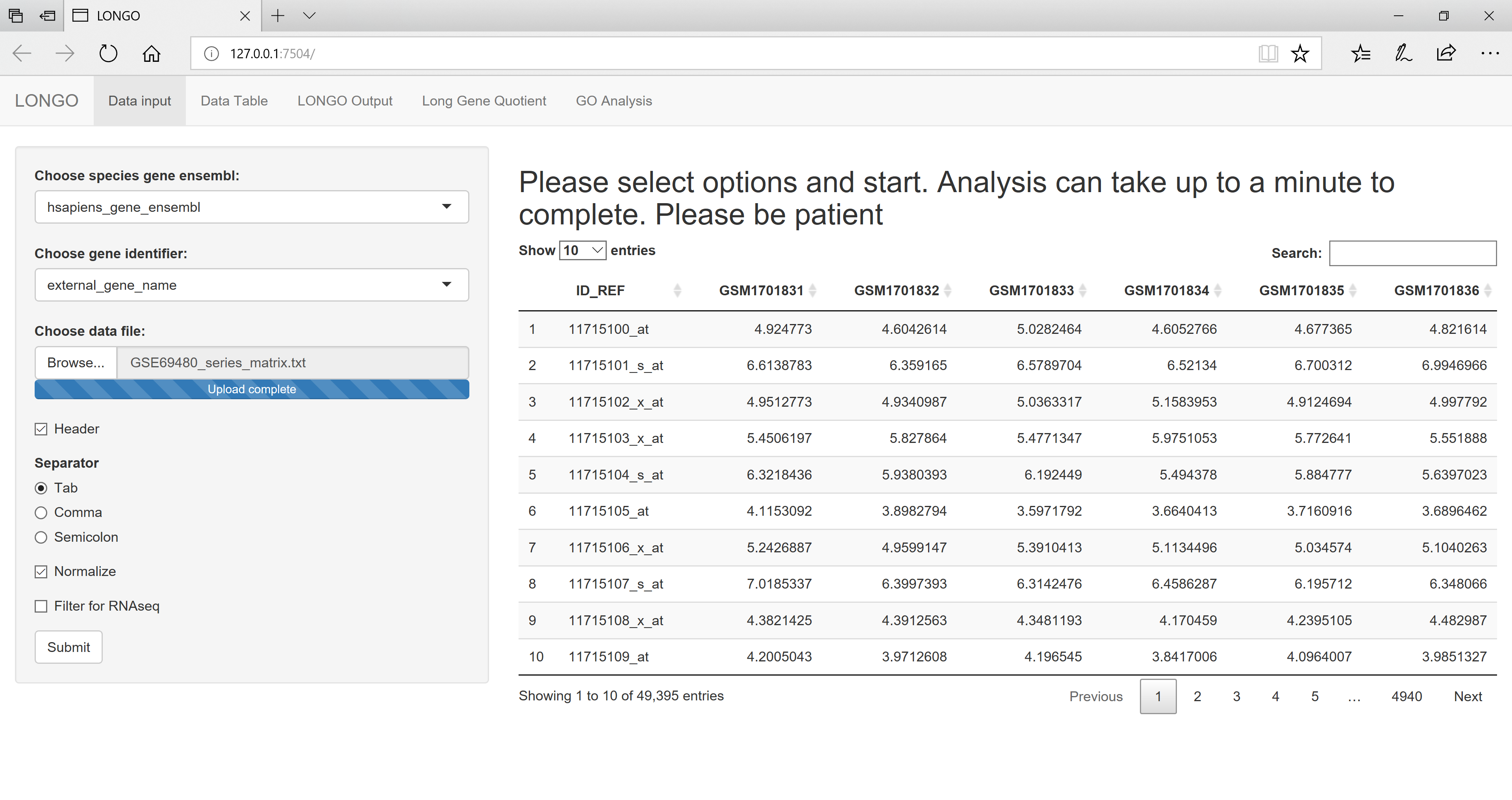
figure 2

This next step can take up to a minute depending on how large the dataset is. Once LONGO finishes there will be a notice on the top stating it completed and the time it finished. The Data Table tab shows the results of the gene names and gene lengths depending on the gene identifier used. There is an option to download this data.

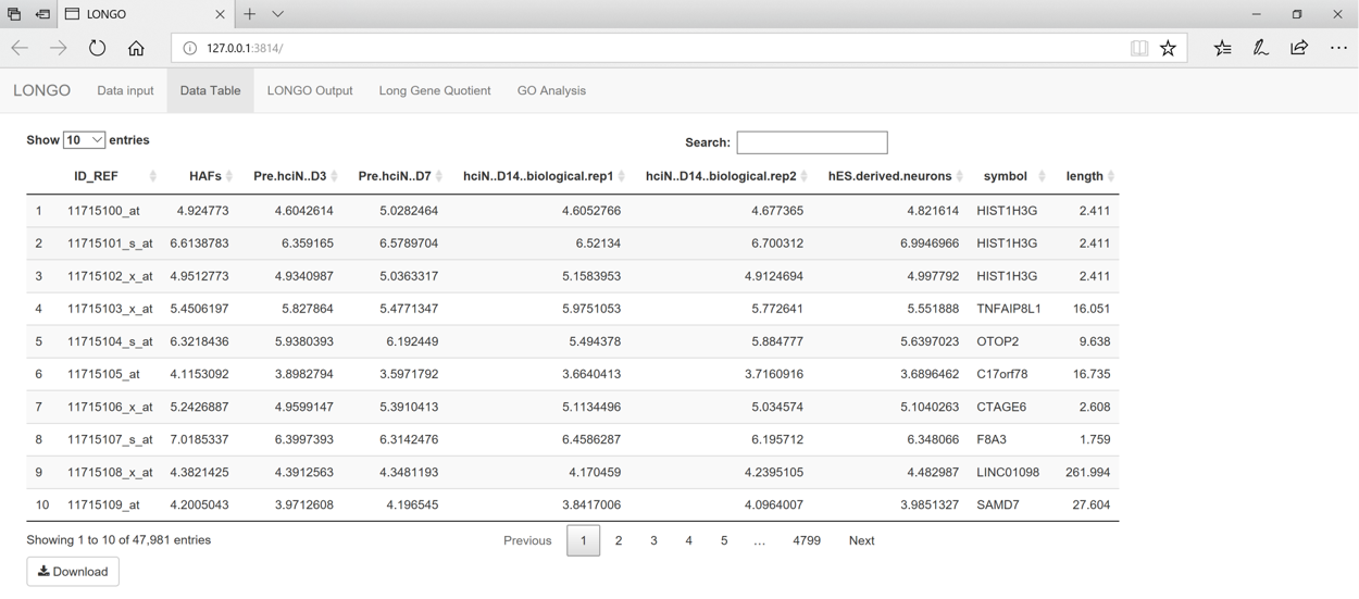
figure 3

The LONGO Output tab shows the LONGO plot. This plot shows the results of the window binning for each dataset. The initial results are using the default values.

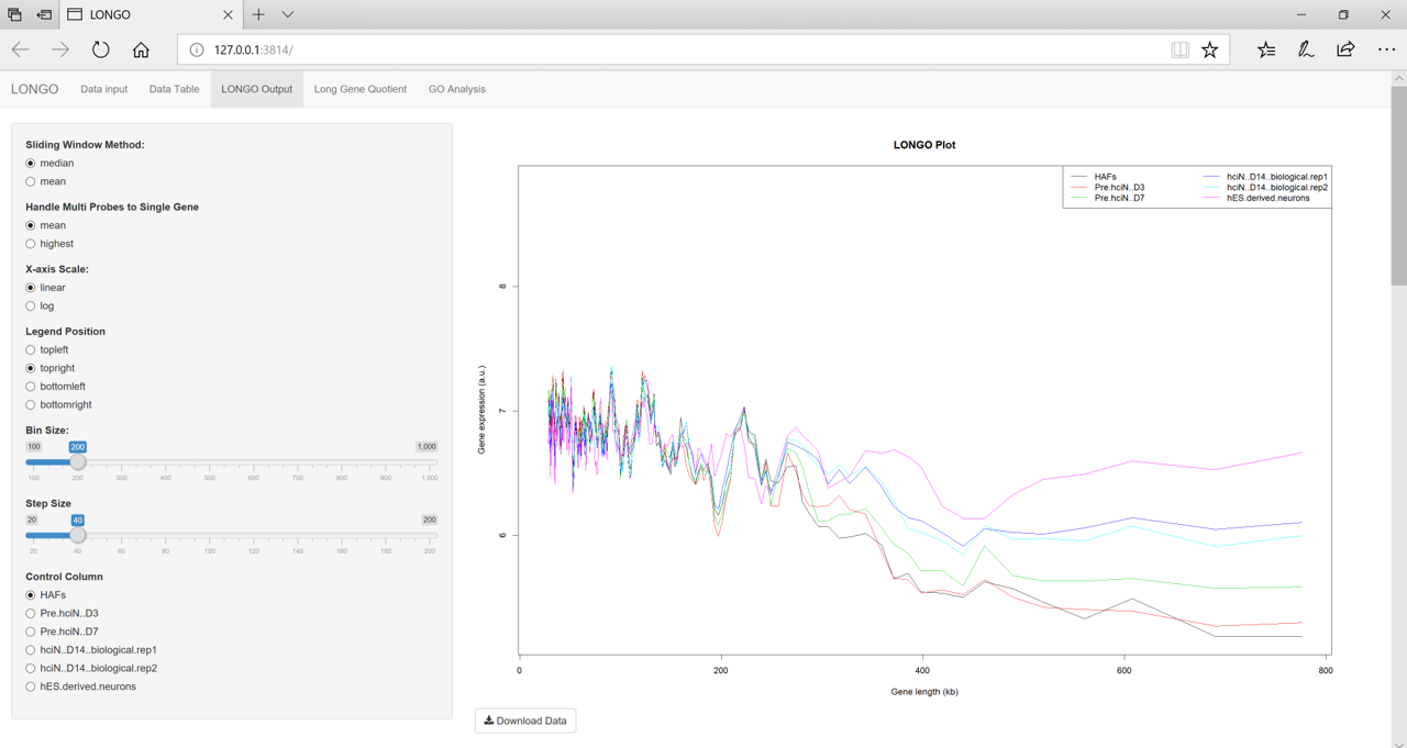
figure 4

There are several parameters on the side panel of the LONGO Output tab. All of these options change the results.

• Sliding Window Method This parameter is used to get the final bin result. The two options median or mean can be used. The median is the default option which takes the median expression of all the genes within the window.
• Handle Multi Probes to Single Gene This parameter is used to reduce the number of gene identifiers which are for the same gene. There are two options the mean or the highest.
• X-axis scale This parameter is used as the axis for the plots.
• Legend Position This parameter changes the position of the legend.
• Bin Size This parameter is used change the size of the bin. The default is 200. Dencreasing the bin size, increases the chances of a bin not having any genes. This will mess up the plot.
• Step Size This parameter is used to change the step size LONGO takes.
• Control Column This parameter is used if the data has a control column in your data. This option is used for calculating the LONG Gene Quotient.

The Long Gene Quotient tab shows the bar graph with the results of the Long Gene Quotient analysis. The red bar is used to mark the 0.25 point. Generally any LQ value above 0.25 means the sample is neuronal.

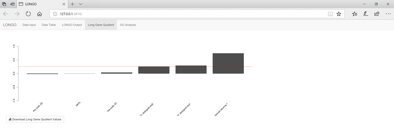
figure 5

The GO Analysis tab allows creation of a GO enrichment graph using the topGO package. There are multiple input variables that can be altered to get different graphs. - Domain for GO Analysis This parameter is used to determine which Gene Ontology Domain should be used: Cellular Component, Molecular Functions, Biological Processes. - GO Scoring Method - GO Graphing Method - Number of Significant Node to Graph - P-value for significance - Scale for Graph Text - Replicates - Number of Treatments This is used to determine how many options will be displayed for the samples

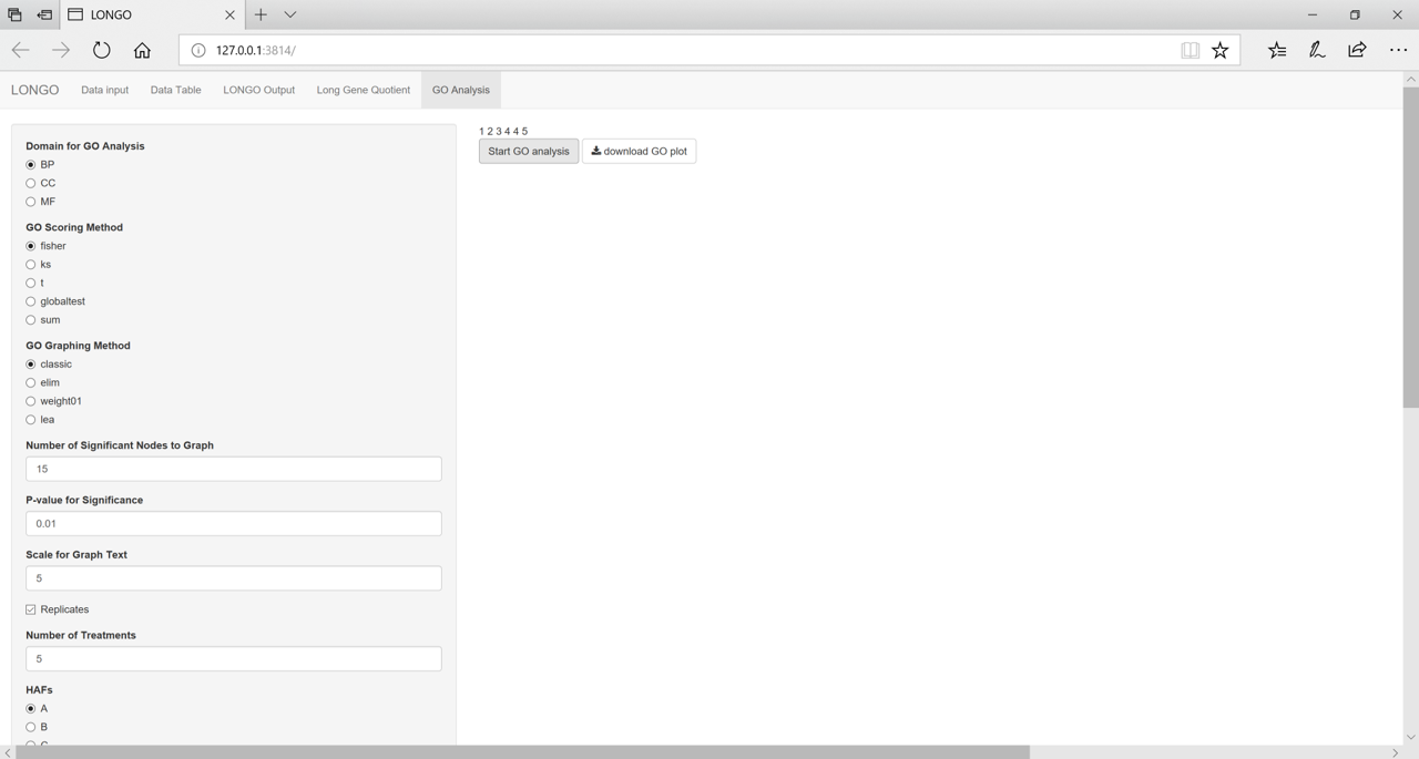
figure 6

LONGOcmd():

The LONGOcmd function will automatically write the output data files to your working directory. This can allow faster data analysis if you know the values to use. LONGOcmd can also be used with an R dataframe as the input file as long as it satisfies the format described in the pre-processing section above. The shiny interface is more beginner friendly while the LONGOcmd() requires more specific knowledge at the start. The LONGOcmd() function uses the same techniques but requires only the initial input. If you know the BioMart species database and gene identifier, you can use this for faster analysis. The first example gives an overview of the possible input variables and their defaults. The other examples use a data file that is included in the LONGO package.

    LONGOcmd(fileLocation = path_to_file, {separator = ","},
        {header = TRUE}, {commentChar = "!"},
        {species = "hsapiens_gene_ensembl"}, 
        {libraryType = "affy_primeview"}, {multiProbes = "mean"},
        {windowSize = 200}, {stepSize = 40}, {windowStyle = "mean"},
        {filterData = TRUE}, {normalizeData = TRUE}, {controlColumn = 2})
            
    LONGOcmd(exampleRatData, SPECIES = "mmusculus_gene_ensembl",
        LIBRARY_TYPE = "external_gene_name")
    
    LONGOcmd(exampleRatData, SPECIES = "mmusculus_gene_ensembl",
        LIBRARY_TYPE = "external_gene_name", WINDOW_SIZE = 350, 
        MULTI_PROBES = "highest", FILTERED = FALSE)

Biomart identifier options (as of 2018-03-09)

Below is a list of all the Biomart data sets available.

##                           dataset
## 1         cchok1gshd_gene_ensembl
## 2          csyrichta_gene_ensembl
## 3     aplatyrhynchos_gene_ensembl
## 4            hfemale_gene_ensembl
## 5         ccapucinus_gene_ensembl
## 6              catys_gene_ensembl
## 7      dnovemcinctus_gene_ensembl
## 8             fcatus_gene_ensembl
## 9          ppaniscus_gene_ensembl
## 10          saraneus_gene_ensembl
## 11            rbieti_gene_ensembl
## 12         oanatinus_gene_ensembl
## 13             hmale_gene_ensembl
## 14       fdamarensis_gene_ensembl
## 15         ecaballus_gene_ensembl
## 16         pvampyrus_gene_ensembl
## 17           sscrofa_gene_ensembl
## 18           mpahari_gene_ensembl
## 19        oniloticus_gene_ensembl
## 20        tbelangeri_gene_ensembl
## 21        cpalliatus_gene_ensembl
## 22            oaries_gene_ensembl
## 23         csavignyi_gene_ensembl
## 24           ngalili_gene_ensembl
## 25         psinensis_gene_ensembl
## 26        eeuropaeus_gene_ensembl
## 27           ggallus_gene_ensembl
## 28       scerevisiae_gene_ensembl
## 29          mmulatta_gene_ensembl
## 30        gaculeatus_gene_ensembl
## 31          tguttata_gene_ensembl
## 32       xtropicalis_gene_ensembl
## 33          neugenii_gene_ensembl
## 34         mmusculus_gene_ensembl
## 35           pabelii_gene_ensembl
## 36        lchalumnae_gene_ensembl
## 37         etelfairi_gene_ensembl
## 38         clanigera_gene_ensembl
## 39            dordii_gene_ensembl
## 40          hsapiens_gene_ensembl
## 41          csabaeus_gene_ensembl
## 42          olatipes_gene_ensembl
## 43     mfascicularis_gene_ensembl
## 44        cporcellus_gene_ensembl
## 45        choffmanni_gene_ensembl
## 46           panubis_gene_ensembl
## 47        ogarnettii_gene_ensembl
## 48        xmaculatus_gene_ensembl
## 49         loculatus_gene_ensembl
## 50     tnigroviridis_gene_ensembl
## 51        mgallopavo_gene_ensembl
## 52        amexicanus_gene_ensembl
## 53          mauratus_gene_ensembl
## 54            drerio_gene_ensembl
## 55     cintestinalis_gene_ensembl
## 56         sharrisii_gene_ensembl
## 57       mnemestrina_gene_ensembl
## 58       falbicollis_gene_ensembl
## 59         lafricana_gene_ensembl
## 60         trubripes_gene_ensembl
## 61      ptroglodytes_gene_ensembl
## 62          cjacchus_gene_ensembl
## 63          ggorilla_gene_ensembl
## 64        mdomestica_gene_ensembl
## 65      sboliviensis_gene_ensembl
## 66         mspreteij_gene_ensembl
## 67      mochrogaster_gene_ensembl
## 68 itridecemlineatus_gene_ensembl
## 69          mmurinus_gene_ensembl
## 70         pcapensis_gene_ensembl
## 71       cfamiliaris_gene_ensembl
## 72            odegus_gene_ensembl
## 73       rnorvegicus_gene_ensembl
## 74          jjaculus_gene_ensembl
## 75          pformosa_gene_ensembl
## 76        ttruncatus_gene_ensembl
## 77          celegans_gene_ensembl
## 78         oprinceps_gene_ensembl
## 79           gmorhua_gene_ensembl
## 80     acarolinensis_gene_ensembl
## 81             mfuro_gene_ensembl
## 82          pbairdii_gene_ensembl
## 83      mleucophaeus_gene_ensembl
## 84        mlucifugus_gene_ensembl
## 85           ccrigri_gene_ensembl
## 86          pmarinus_gene_ensembl
## 87           btaurus_gene_ensembl
## 88        rroxellana_gene_ensembl
## 89     dmelanogaster_gene_ensembl
## 90      amelanoleuca_gene_ensembl
## 91        ocuniculus_gene_ensembl
## 92           caperea_gene_ensembl
## 93        pcoquereli_gene_ensembl
## 94            vpacos_gene_ensembl
## 95       nleucogenys_gene_ensembl
## 96           mcaroli_gene_ensembl

Once the data set is selected from above it is possible to get a list of possible gene identifies using the following command, where ‘speciesDataset’ is a data set from the above list.

    ensembl <- biomaRt::useMart("ENSEMBL_MART_ENSEMBL", 
        host = "www.ensembl.org", dataset=<speciesDataset>)

For the LONGO analysis, the “external_gene_name” from the BioMart data set was used as the source of the gene name. This was used to determine if there were duplicate reads. The method for handling these repeats is based on the input variable of “MULTI_PROBES”